Current Examples
This demo is implemented in a single Python file. Download here: tutorial_current.ipynb
This demo illustrates how to:
Define currents in the electrodes.
from module1_mesh import*
from module2_forward import*
from module3_inverse import*
from module4_auxiliar import*
import matplotlib.pyplot as plt
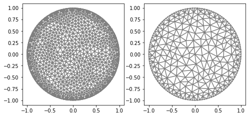
Mesh
mesh_inverse, mesh_direct=MyMesh(r=1, n=8, n_vertex=121)
plt.figure(figsize=(8, 8))
plt.subplot(1,2,1)
plot(mesh_direct);
plt.subplot(1,2,2)
plot(mesh_inverse);
Current Examples
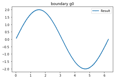
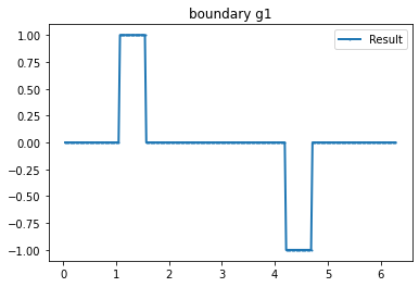
Method 1
"Current"
n_g=3 #Number currents
I_all=current_method(n_g, value=1, method=1) #Creating current

#Plotting
for i in range(n_g):
        mesh=mesh_direct
        VD=FiniteElement('CG',mesh.ufl_cell(),1)
        g_u=interpolate(I_all[i], FunctionSpace(mesh,VD))
        g_u=getBoundaryVertex(mesh, g_u)
        bond=plot_boundary(mesh, data=g_u, name='boundary g'+str(i))
>>> print("Mesh Direct:")
>>> Verifyg(I_all, mesh_direct)
>>> print("\n Mesh Inverse:")
>>> Verifyg(I_all, mesh_inverse)

Mesh Direct:
Integral boundary: 2.42861286636753e-16 0
Integral boundary: -1.3357370765021415e-16 1
Integral boundary: -3.122502256758253e-16 2
Integral boundary g(0)*g(1): 0.0
Integral boundary g(0)*g(2): 0.0
Integral boundary g(1)*g(2): 0.0

 Mesh Inverse:
Integral boundary: 3.469446951953614e-18 0
Integral boundary: -9.020562075079397e-17 1
Integral boundary: -3.469446951953614e-17 2
Integral boundary g(0)*g(1): 0.0
Integral boundary g(0)*g(2): 0.0
Integral boundary g(1)*g(2): 0.0
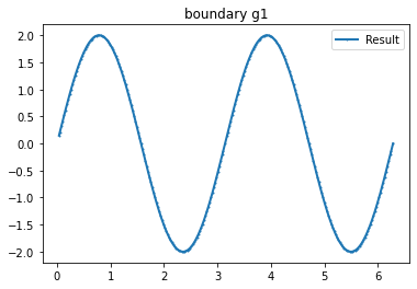
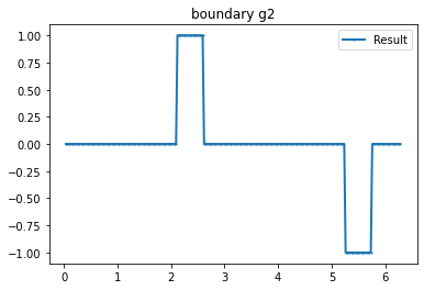
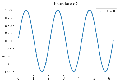
Method 2
"Current"
n_g=3 #Number currents
I_all=current_method(n_g, value=1, method=2) #Creating current

#Plotting
for i in range(n_g):
        mesh=mesh_direct
        VD=FiniteElement('CG',mesh.ufl_cell(),1)
        g_u=interpolate(I_all[i], FunctionSpace(mesh,VD))
        g_u=getBoundaryVertex(mesh, g_u)
        bond=plot_boundary(mesh, data=g_u, name='boundary g'+str(i))
>>> print("Mesh Direct:")
>>> Verifyg(I_all, mesh_direct)
>>> print("\n Mesh Inverse:")
>>> Verifyg(I_all, mesh_inverse)

Mesh Direct:
Integral boundary: 8.270294171719428e-16 0
Integral boundary: 4.163336342344337e-16 1
Integral boundary: -3.469446951953614e-17 2
Integral boundary g(0)*g(1): 1.0598076236045806e-17
Integral boundary g(0)*g(2): 0.0010576671174781075
Integral boundary g(1)*g(2): 4.217546450968612e-17

 Mesh Inverse:
Integral boundary: 7.4593109467002705e-16 0
Integral boundary: -2.7582103268031233e-16 1
Integral boundary: 3.122502256758253e-17 2
Integral boundary g(0)*g(1): 3.8294020732188017e-16
Integral boundary g(0)*g(2): -7.741203511546502e-17
Integral boundary g(1)*g(2): -4.85722573273506e-17
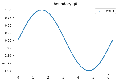
Example 1
myI1=Expression(" sin(x[0]*pi) ",degree=2)

   g_u=interpolate(myI1, FunctionSpace(mesh,VD))
   g_u2=getBoundaryVertex(mesh, g_u)
   bond=plot_boundary(mesh, data=g_u2, name='boundary g')
>>> Verifyg([g_u], mesh_direct)
Integral boundary: -1.4991805540043313e-16 0
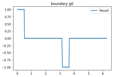
Example 2
myI2=Expression(" x[1]>0 ? 1 :-1 ",degree=1)

g_u=interpolate(myI2, FunctionSpace(mesh,VD))
g_u2=getBoundaryVertex(mesh, g_u)
bond=plot_boundary(mesh, data=g_u2, name='boundary g'+str(i))
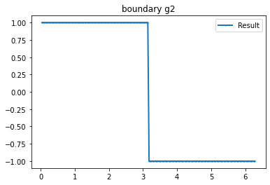
>>> print(assemble(g_u*ds(mesh))) #Integral boundary #Like Verifyg
-1.6306400674181987e-15
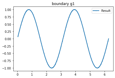
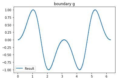
Example 3
value=2
n_g=2

myI3=[Expression(f" x[1]>=0 ? {value}*sin(acos(x[0])*{i+1}) : {value}*sin((-acos(x[0]))*{i+1})",degree=1) for i in range(0,n_g)]

for i in range(n_g):
    mesh=mesh_direct
    VD=FiniteElement('CG',mesh.ufl_cell(),1)
    g_u=interpolate(myI3[i], FunctionSpace(mesh,VD))
    g_u2=getBoundaryVertex(mesh, g_u)
    bond=plot_boundary(mesh, data=g_u2, name='boundary g'+str(i))